Read mapping

Note

Considering DNA sequencing data (WGS or ES), referenced-base assembly often follows the goal of finding the differences between an individual’s genome and the reference genome for the corresponding species, rather than characterising the genome of that species in the first place.

Reads being aligned/mapped to the reference genome are a prerequisite for variant calling, the computational identification of high quality mutations from sequencing data.

Search algorithms like Smith-Waterman are quite slow, but faster search algorithms based on preprocessing of the text to build a substring index exist. A substring index is a data structure which gives substring search in a text or text collection in sublinear time.

Naive string search

Given a genome with characters and read of characters, the simplest string algorithm would simply slide the pattern across the genome, extending it letter for letter as long as there is a match, with .

Trie

Note

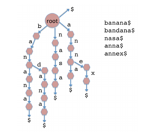
A trie (from retrieval), is a multi-way tree structure useful for storing strings over an alphabet. It’s defined as the smallest tree over an alphabet such that each edge of the trie is labelled with one character , a node has at most one outgoing edge labelled for each (at most ), and each key is spelled out along some path starting at the root.

$ is a symbol that does not appear anywhere in our genome template , we define it to be lexycografically less than our other characters, therefore the $ enforces a lexicographic rule that we know from dictionaries (for instance, “over” comes before “overture”). The $ also ensures that no suffix will be considered as a prefix of any other suffix.

If is the maximum length of any read, then the runtime of the trie algorithm is for matching and for trie construction, where is the combined length of our reads. This is quite time efficient, however the amount of memory required for the trie is in the worst case proportional to the total length of the reads, which can be enormous .

Suffix Tries

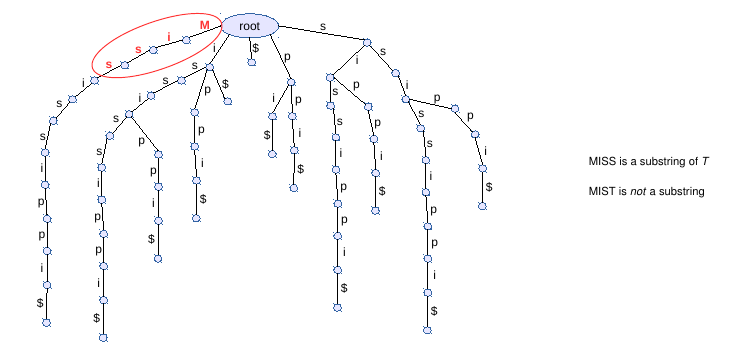
Instead of using different words for the trie, let’s use suffixes of $, hence, each path from the root to a leaf represents a suffix, and each suffix is represented by a path from the root to a leaf.

Each substring is represented by a path from the root, because every substring is a prefix of some suffix of . Thus to search for a substring , start at the root and follow the edges labelled with the characters of . If at some point there is no outgoing edge for the next character of , then is not a substring of .

To construct a suffixTrie we use the following algorithm:

SuffixTrie(T):
	T += $
	root = {}
	for i <- 1 to length(T)
		n = root	# n is the current node
		for c in T[i:]	# for each char in the i-th suffix
			n[c] = {}	# add outgoing edge to n if needed
		
		n = n[c]	# switch current node to child node
	
	return root

The followPath algorithm returns the node at the end of the path or NULL if there is no path:

followPath(T, S):
	root = SuffixTrie(T)
	n = root	# n is the current node
	for i <- 1 to length(S)
		c = S[i]	# i-th char of S
		
		if c not in n then
			return NULL	# not found
		
		n = n[c]	# switch current node to child node
	
	return n

The hasSubstring algorithm checks if followPath does not “fall off” the tree and returns NULL:

hasSubstring(T, S):
	return followPath(T, S) != NULL

Suffix Trees

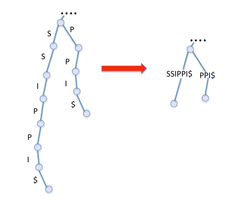
Given , the worst case for space complexity is , that is too large. To optimise this we can combine non branching paths into a single edge with a string label:

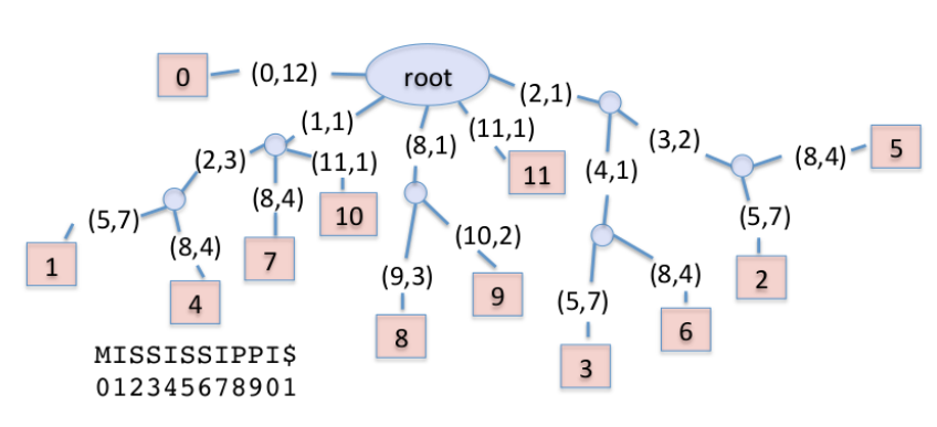
By doing this we make sure that our tree has at most as many internal nodes as a full binary tree, because if an internal node has more than children we have fewer parent nodes, thus there are less or equal to total nodes, so . This works but the total length of the edge labels is still . To reduce size complexity further we can store in each edge only the offset and length of the original labels in the original string, so there are only two integers for one edge ().

This is a Suffix Tree, and we can also build it directly using Ukkonen’s linear time on-line suffix tree construction algorithm.

To fine all matches of a sequencing read in a genome , letting be the number of matches and be the length of , the search is then .

Suffix trees, although having a linear algorithm has a really high constant factor ( means ), therefore it can be quire impractical.

Suffix arrays

Note

The suffix array, at leas in its simplest incarnation, requires only per character of the input sequence.

Given a string , the suffixes of this strings are:

A naive implementation of the suffix array basically manipulates an array of pointers to the suffixes of .

A naive approach to build a suffix array is:

1. Form all possible suffixes from the input string , and with each suffix associate it’s position/index in the original string
2. Sort lexicographically to bring repeated strings together, we only keep the index array

Manber and Myers algorithm

The naive approach to build the suffix array is not very efficient, the Manber and Myers algorithm has . It works by:

1. Sorting only the first character of the suffixes (using key-indexed counting sort)
2. Recursive phase (): given an array of suffixes sorted on the first characters, create an array of suffixes sorted on the first characters

Burrows Wheeler Transform

Note

The Burrows Wheeler Transform (BWT) applies a reversible transformation to a block of input text. The transformation itself does not compress the data, but reorders it to make it easy to compress with simple algorithms.

To make the BWT of a input text :

1. Form all rotations of the input text , appended with the $
2. Sort the rotated strings lexicographically, the result is the Burrows Wheeler matrix
3. The BWT is simply the last column of the Burrows Wheeler matrix

We denote the BWT of an input string as:

BWT from Suffix Array

The Burrows Wheeler matrix is nearly the same as the suffixes referred to by the suffix array of the same string.

We can now write an algorithm to create from the suffix array of by noting that position of the BWT corresponds to the character that, in the original string, is just to the left of the -th suffix in the SA.

We can now create the BWT as follows:

The naive algorithm for this:

bwtFromSuffixArray(T):
  sa = constructSuffixArray(T$)
  L = length(sa)
  bwt = new string[L]
  
  for i <- 0 to L - 1
  	if sa[i] = 0
  		bwt[i] = $
  	else
  		bwt[i] = T[sa[i] -1]
  	
  	return bwt
  	```

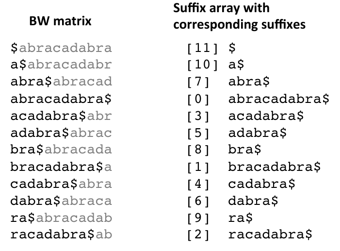
LF Mapping property

For any character, the -ranking of characters in the first column of the BW matrix is the same as order of characters in the last column .

The -ranking of the character at any given position is the number of times that an identical character has preceded it in .

The -ranking of a character at a specific position is the number of times the character has occured in the column above the current position.

The reversibility of the BWT depends on the LF Mapping property. We can reverse the BWT by following this visual algorithm:

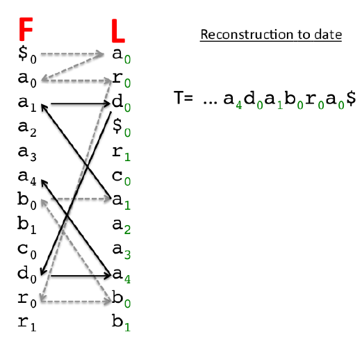
Note that we can do this process starting only from the , which corresponds to the column, if we count the number of each character in , we can easily reconstruct the chunks of characters in the column of the BWM, using the cumulative index property.

FM Index

Note

The Full-text index in Minute space (FM index) uses the BWT and some other auxiliary data structures to generate a fast and efficient index for small patterns within a larger string .

The main data structures are the and column from the BWM. Note that the column itself is not stored because it can be represented as an array of integers.

Given a string to be searched in our genome , we look for all the rows that start with the last letter of in , we then look in to identify those rows whose last letter corresponds to the second to last letter in , we now use the LF mapping to find the rows in that begin with these characters.

If no letters can be found in , the search pattern doesn’t exist in .

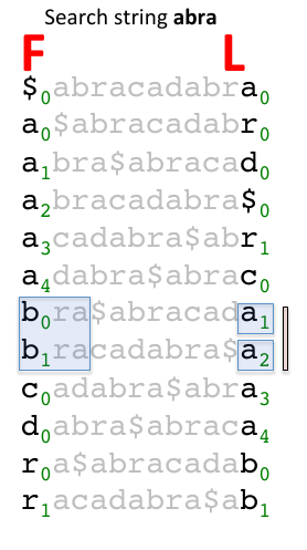
The naive implementation of the algorithm has many problems:

• We need to find the preceding characters efficiently, at the worst case this has
• We still need a way to get the -ranks of the characters in
• We still need a way of figuring out at what positions matches occur in

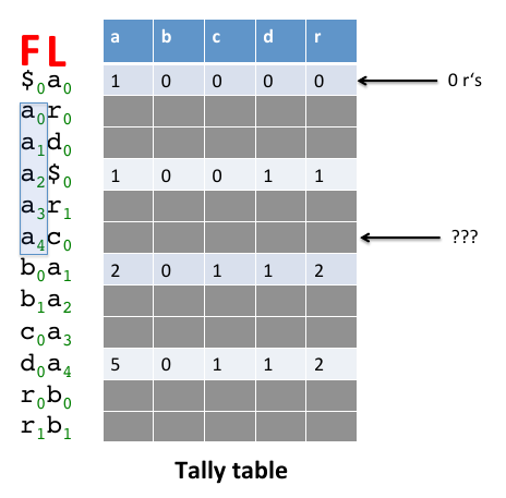
To fix these issues we construct a tally table that precalculates the number of each specific character in up to every row.

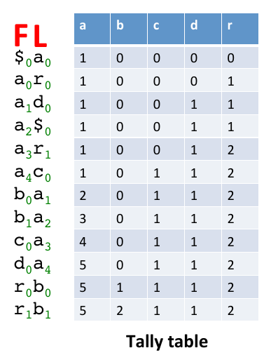
After we found all rows beginning with the last character of , we need to find rows with the second to last character in the column. Say the range of rows is , we look in the tally table in row and in row . We now know how many characters occur in , in that range, therefore there are only that many lookups instead of .

This approach however needs to store integers, therefore we store only at every -th row.

This also provides us with the -ranks, if we subtract from the tally. Finally, to find the position of the match we can use a similar approach, taking advantage of the LF mapping.

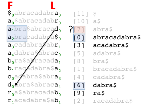
BWT/FM Index algorithms for read mapping

There are lots of published read aligners for genomic resequencing. Perhaps the best known amongst them use the BWT/FM Index plus lots of bells and whistles.

Burrows Wheeler Aligner

Note

BWA is an algorithm based on BWT, that takes into account inexact matching.

Let be two strings over the alphabet , let and , let be the distance measure between two strings and , let be a threshold for the maximum allowed distance, and finally let be the substring of having length starting at position .

Prefix trie

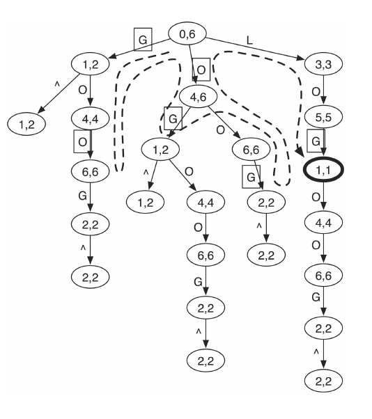
Let’s consider the prefix trie for the string , that is equivalent to a suffix trie but a path from a leaf to the root gives a unique prefix of .

Like for BWT, we start searching for substrings with the last character of the substring using DFS, and for inexact matching we bruteforce it to allow for up to mismatches.

Suffix array interval

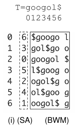
All occurrences of a substring in the original string appear next to each other in the suffix array, because a substring is equivalent to the prefix of a suffix of and we have lexicographically sorted all suffixes, therefore a substring can be represented as a SA interval:

The BWA paper presents the method for calculating the SA interval of the query word that we’ve already seen.

To inexact search over a suffix array we use the algorithms:

InexactSearch(W,z):
	CalculateD(W)	# Precalculates lower bounds of the number of mismatches
	# returns the SA intervals of substrings in T that match W with no more than 
	# z differences
	return InexRecur(W, |W| - 1, z, 1, |T| - 1)

CalculateD(W):
	z <- 0
	j <- 0
	for i = 0 to |W| - 1
		if W[j ... i] is not a substring of T
			z <- z + 1
			j <- i + 1
		
		# sets the lower bound of the number of differences in W[0 ... i] to
		# the best match T
		D(i) <- z
	
	return D

InexRecur(W, i, z, k, l):
	if i < 0
		return { k, l }	# for instance a SA interval
	
	if z < D(i)
		return { }
	
	l <- { }
	
	for b in { a, c, g, t }
		k <- C(b) + O(b, k - 1) + 1
		l <- C(b) + O(b, l)
		
		if k <= l
			if b = W[i]
				l <- l union InexRecur(W, i - 1, z, k, l)	# match
			else
				l <- l union InexRecur(W, i - 1, z - 1, k, l)	# mismatch
	
	return l