Note
We need to model DNA sequences to do things such as make some hypotheses about it, build a generative model to descrive it or find sequences of similar type (in terms of characteristics).
Goals of sequence modeling include:
- The ability to emit DNA sequences of a certain type
- The ability to recognise DNA of a certain type
- Ability to learn distinguishing characteristics of each state
An alignment profile/motif is a model for a specific DNA pattern, however this isn’t really practical since all other instances of the pattern are assumed to have the same length
Once defined the model, we can employ it to find other instances of the pattern in new sequences.
Sequence modeling is probabilistic, and we use tools such as Markov Chains and Hidden Markov Models (HMMs) to model sequences.
Markov chains and Hidden Markov Models
Note
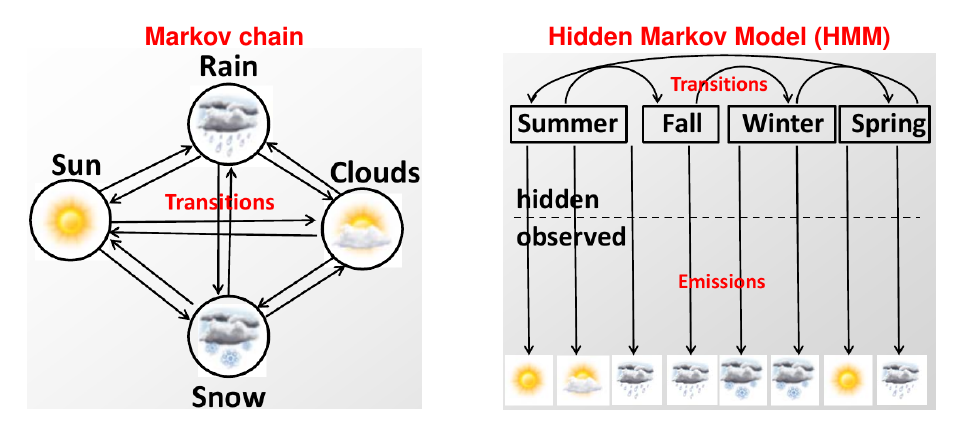
A Markov chain is a sequence of data items generated by a model which has one state (node) per symbol/letter and certain transition probabilities between the edges.
In a Hidden Markov Model the model transitions between different states like in a Markov Chain, however the states are not directly observable. Instead, each state has associated emission probabilities to generate certain observable data items.
In other words, we don’t know in which state the model is in, we can only observe which characters the model is emitting.
We define the transition probability from hidden state
to hidden state : The emission probability of symbol
when the hidden state is : The hidden path (sequence of hidden states of a set
): The sequence of observations of a set
of symbols: The transition matrix that maps the probability of
state transitions: The emission vector that represents the probability of observing the possible observable letters
from state :
Definition of a Markov Chain
A Markov chain is a triplet
where is a finite set of states, where each state corresponds to a symbol in the alphabet , is a vector of initial state probabilities, and is the matrix of state transition probabilities. The output of the model is the state at each instant time.
The probability of each observed symbol
depends only on the value of the preceding symbol : Therefore the probability of observing a specific sequence
of length is: Where
is the initial state of probability of .
Definition of a Hidden Markov Model
A HMM is a
-tuple is a finite set of states, where each state corresponds to a symbol in the alphabet , is a finite set of observable symbols ( ), is a vector of initial state probabilities, is the matrix of state transition probabilities, and is a emission probability matrix with Both emissions and transitions are dependent on the current state only and no on the past.
A typical representation of a process which can be modelled by a HMM includes:
- Start: a random initial state
according to the initial state probabilities - The random choice to move from the current state
to the next state that depends on transition probabilities - For each step
of the hidden path, the hidden state randomly emits an observable symbol according to the emission probabilities
The probability of observing
HMM in the context of DNA
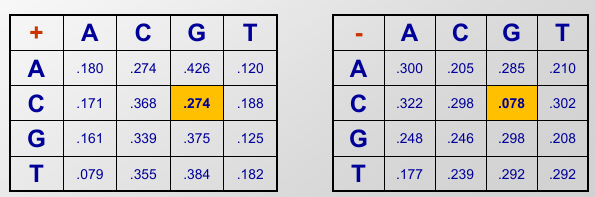
In biology the order of letters matters. A “C” followed by a “G” (often written as CpG) is incredibly important, because “CpG islands” usually mark the start of a gene. If the computer can’t remember the previous lettere, it can’t find these islands.
To fix this, scientists expand the HMM state space, by weaving the memory directly into the labels. Instead of having just one generic state for the letter “G”, they create unique states that look backward:
Where the
marks the base as inside a CpG island, while the marks the base as outside one. The transition probabilities are show below:
Decoding
Note
Given the model parameters
and , and a sequence of emissions we can find the sequence of hidden stats using the Viterbi algorithm. We define
as the probability of the most likely path through state , and we compute: We need to find the path
that maximises the total join probability . Assuming we know for the previous time step, we can calculate:
We initialise
and . Calculating iteratively the previous value, and following max pointer back we can find: This algorithm has a time complexity of
and a space complexity of .
Evaluation
Note
Given the model parameters
and , and a sequence of emissions we can find the total probability of generating a given over any path, that is: To calculate it we define the forward probability as:
Assuming we know
for the previous time step, we can calculate:
We initialise
and . We then calculate: This algorithm has a time complexity of
and a space complexity of .
Posterior decoding
Note
To find the likelihood that an emission
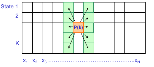
is generated by a state in a specific position, we can use posterior decoding, that looks at the entire DNA sequence to decide what is happening in a specific position. To do this it has to calculate and add up every single possible path that could have led to that base, and every path that could follow it: To calculate the backward probability we compute:
By initialising
, we can compute: This algorithm has a time complexity of
and a space complexity of . We can then evaluate:
We also define
.
Supervised learning
Note
Given a string of DNA, where every single CpG island is explicitly highlighted, it’s possible to use supervised learning to train a model with basic parameters. Given
, and , we can show that the maximum likelihood parameters are:
Given very little data, there may be overfitting, that means those formulas may say the probability is
Unsupervised learning
Note
Sometimes we may not know the true values of
and , and we may not know where CpG islands are. To fix this, we estimate our “best guess” on what those values are, using maximum-likelihood estimation, we update the probabilistic parse of our sequence based on these parameters, and we iterate.
Viterbi Training
The Viberbi training approach performs Viterbi to find
, it calculates and according to , and then calculates the new parameters . This is repeated until convergence.
Baum-Welch Algorithm
The Baum-Welch algorithm picks the best guess for model parameters, and then uses the forwards and backwards algorithms to calculate a weighted average across all possible paths. It then calculates
and , and calculates the new model parameters and . This is repeated until doesn’t change much. This has a time complexity of:
And it’s not guaranteed to find globally best parameters.