Multiple sequence alignment

Note

Many applications (especially in the field of evolutionary genetics/genomics) it’s useful to align multiple sequences to each other at the same time.

Formally, a Multiple Sequence Alignment (MSA) of strings over an alphabet is a set of strings with gaps "" over the alphabet where:

The possible ways to align strings depend on where we place gaps.

Given this definition it’s always possible to find a “consensus”, which is exactly the common ancestor word.

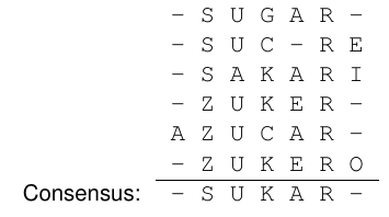
Multiple sequence alignment can give us much more information, and a more general view of what the relationships among all our sequences are.

Sum of pairs

The possible ways to align strings depend on where we place gaps. Since multiple alignment implicitly induces a pairwise alignment for every pair , we can use the substitution matrix and compute the pairwise alignment for every pair. We can then compute the sums of pair:

The SP score is essentially a generalisation to strings of the principle we applied to strings.

Neighbouring cells

Note

The optimal solution can also be found by dynamic programming, using a -dimensional hypercube, where the last cell in the structure will contain the score of the optimal multiple alignment.

A cell has . For , we can then use:

Where is an entry in the 3D scoring matrix. Each step is one column in the alignment, so we can compute the corresponding :

We then need a 2D scoring matrix for alignment matches, to compute and a gap penalty. Also we set because aligning two gaps has little meaning from a biological point of view.

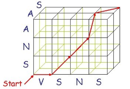
This algorithm has a space complexity of , and a time complexity of , therefore this problem is NP hard.

NP Hard problems

When we face a NP hard problem, we have to find a way to solve it anyway. There are different possibilities:

• Changing the formalisation
• Explore the space of possible solutions, considering only a reasonable polynomial subset of them, hoping that it contains the optimal solution
• Design a polynomial time/space algorithm, based on some heuristic hoping to find the optimal solution
• Design an approximation algorithm

Suppose that we design a polynomial time algorithm for an NP hard maximisation problem. For instance of the problem, let be the value of the solution found, while let be the optimal maximum value for instance . If we can prove that:

Then we have a performance guaranteed approximation algorithm.

Of course we want to be as close as possible to .

Center star algorithm

Note

Given an input of strings , we compute the pairwise alignment of every pair of input strings. Let be the score of the alignment of strings and , and let be the total pairwise alignment score of with all other strings. We then choose to be:

We call this the center of the star. The multiple alignment is built by starting with and iteratively adding the other strings as they were aligned to in step .

Overall, the space/time complexity equals to .

Approximation

To approximate the Center star algorithm, we just compare all the strings to the center, hoping that the pairwise alignment of each of them would also be found in the optimal multiple alignment.

By minimising the overall distance instead of the maximising the overall similarity, if the triangle inequality holds (for edit distance it does), we can prove that it’s an approximation algorithm with .

Alignment profile

Note

One useful way to describe a multiple alignment is to represent it as an alignment profile. For each column of the alignment, the profile represents the frequency with which we find each symbol of the alphabet (including the gap) in that column, where frequencies in each column sum up to .

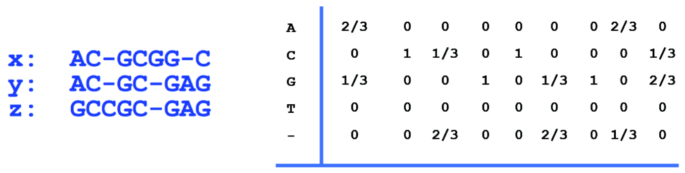
We can add another sequence to this profile by using a dynamic programming matrix, where we replace one of the strings by an entire profile, where the rows represent the string to be added, while the columns have all letters of the alphabet and their respective frequencies.

We then fill the matrix with a “weighted” version of the global alignment rule.

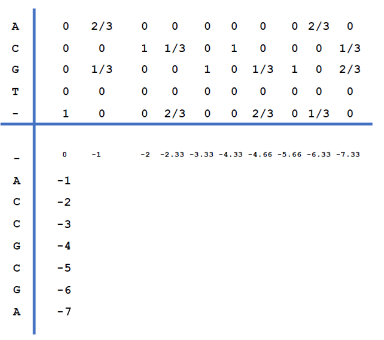
To compute the individual scores for the alignment matrix , given the profile with frequencies for character in column , and given a string to be aligned, we compute the matrix components by using the formula:

Where is the cost of aligning with . Note that . We then update the alignment profile by adding the new string we just aligned and recomputing the new frequencies.

The same principle can be applied to the alignment of two profiles. Also, for global alignment the update of the cells can be performed with a “double weighted” version of the rule.

Guide trees

Note

The idea of progressive alignment is to keep aligning pairs of sequences following their evolutionary history backwards. That is, we start by aligning the strings that are closest relatives, then we move backwards to the more distant history. They key is having the “guide-tree” telling us the order of operations in which the alignment has to be built.

However we need to build the guide tree ourselves.

To do that we start by comparing all sequences and compute their pairwise distances, we choose the pair with minimal distance and build their profile. The alignment represents their common ancestor, and it will be part of the final multiple alignment. We repeat this process iteratively until we get a common ancestor to every string, that way, we constructed the guide tree and the final multiple alignment at the same time. This is actually a hierarchical clustering of the strings.

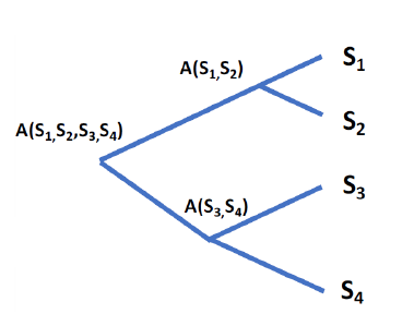
Hierarchical clustering

Hierarchical clustering is one of a set of related data mining techniques.

Where edge length is often depicted proportionally to the computed distance, showing how “close” the individual items and clusters are.

Clustering is a very important branch for data mining, machine learning and statistics, it can be applied to different kinds of data, and each item to be clustered is seen as a point in a multi dimensional space. The data will then be measured with a different distance (or similarity) measures.

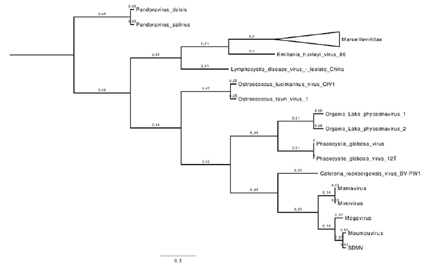
In the guide tree, the distance between two strings is the distance given by their alignment, while the distance between one string and an alignment can be measured by:

• Distance between the string and the closes string of the cluster
• Distance between the string and the furthest string of the cluster
• The average distance between the string and all the strings of the cluster While, for the distance between two clusters:
• Distance of the closest pair of members
• Distance of the furthest pair of members
• Average distance between all pairs of members

For multiple sequence alignment we use neighbour joining, where the measure employed combines the average distance between two objects and the distance of the two objects from all the other objects.

Local multiple alignment

Note

Given a set of input strings , a fixed substring length , and a function for the evaluation of the multiple alignment, we need to find the set of substrings of length , one per input string, that produces the alignment of maximum score according to function .

This problem is also known as “motif finding”.

For motif finding we consider, for each input string we take exactly one substring, all substrings which are part of the solution have the same length , and there will be no gaps in the final solution. Therefore any candidate solution can be simply described by a vector of integers .

We can describe a solution by means of the corresponding profile, with one row per symbol of the alphabet and the frequency of symbol in column . We can then calculate:

We then align every substring of string to every substring of , we obtain a profiles, but we only keep the best profiles, according to their score. Repeating this iteratively gives us a .

Combinatorial optimisation

Note

A solution to the problem is an assignment of a value between and to discrete variables (assuming all strings have length ).

Hence, each candidate solution to the problem can be seen as a point in a -dimensional “search space” of the problem.

In out case there are points that can be visited in the search space.

Local search

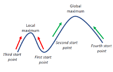
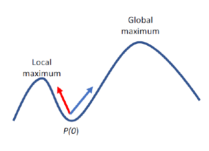
We start at a point in the -dimensional space, chosen randomly or with some heuristic. We then look around at the neighbouring points and compute their scores, and choose the point that will bring the best improvement. We keep moving like this until we find a point at which no further improvement of the objective function is possible. This point is a local maximum.

“Looking around” in the search space at neighbouring points corresponds to changing the value of one or more of the variables in the current solution. One possible way is to select one variable , keeping the other variables fixed and choose the value that brings the best improvement. We iterate this step, by cycling over the variables. This is equivalent to moving in one direction in the -dimensional space, going to the “maximum” point we see in that direction.

This technique is known as “hill climbing”.

A good choice is to iterate the whole algorithm many times with different starting points and output the best solution found across all searches.

Using an approach similar to MAX-CUT we can:

1. Select an
2. Remove the substring corresponding to from the current solution
3. For each , we compute the score by setting and leaving all other variables unchanged
4. Choose such that corresponds to the profile with the highest score
5. Adjust the alignment accordingly and select the next to update

We usually process the variables in random order, using a different random permutation at each cycle, therefore we might get different results even starting from the same initial point. Therefore we iterate several times with different starting profiles.

MAX-CUT

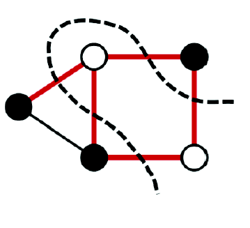
A famous NP hard problem for combinatorial optimisation is the MAX-CUT problem. Given a graph , find the partition of the vertices/nodes into two subsets with such that the number of edges connecting one node of the first partition with one node of the second partition is maximised.

Thus, given vertices, each solution can be described by binary variables indicating to which of the two subsets each node belongs. Therefore is the objective function to be optimised.

To solve this we initialise each binary variable randomly, and variables are updated one by one, from to .

We the iteratively calculate , and if it’s greater then the previous solution it becomes the new solution. This is repeated over all the variables until a complete cycle over all the variables is completed without any improvement.

Stochastic optimisation

In stochastic search, given binary variables, at step , we compare the value with the logical not of its current value, and we the compute:

If we move to the next solution, if not we might accept the change and update the current solution with probability:

Where is a parameter that allows for “fine tuning” the degree of randomness. The value of can be dynamically changed during the execution of the algorithm, for example, we can start with a high value and decrease it at each iteration (thus making the algorithm more and more deterministic).

Applying it to our problem, we have variables defining the substrings’ starting points in the original input, and at step , we choose to replace the value of the variable . For all possible starting positions that the variable can assume we consume the score for each possible , and then we compute the sum of all the scores for all possible substrings for :

We accept a new value for variable with a random choice of probability:

This strategy is known as Gibbs sampling.